Loci
Loci is a declarative C++ framework that simplifies developing large-scale scientific simulations (like CFD) for massively parallel architectures. It was developed by Dr. Ed Luke of Mississippi State University. For more information on Loci, check out the following resources:
Loci is already configured for use in Muscadine. In this demo, we will learn how to load and use Loci on Muscadine for a simple application.
Loading Loci on Muscadine
Loci is exposed via the module system. All required dependencies (GCC, OpenMPI, HDF5, AMD BLIS/LibFLAME, and Scotch) are loaded automatically with the module.
Load Loci:
module load loci/v4.2.a0
Verify that the Loci preprocessor is available:
lpp -v
Setting Up the Demo
For this demo, we will be running the ‘heat’ example module that comes with Loci. We will explore how to load this directory onto your workspace, configure and run it, and finally view the results using Paraview.
Set up a demo folder under your local /scratch directory:
mkdir /scratch/hpc2/$USER/loci_demo
cd /scratch/hpc2/$USER/loci_demo
Copy the heat tutorial directory from source
cp -r $LOCI_BASE/docs/heat/* .
Confirm that you have the following files imported:
╰─$ ls
euler.loci  main.loci  matrix.loci  residual.loci  test.vog
heat.lh     Makefile   plot.loci    test.vars      varFileInputs.loci
Building the Solver
Compile the rule definitions using the pre-configured Makefile:
make # Or use `make -j64` or similar to speed this up
lpp compiles the .loci rule definitions into standard C++ and links against libLoci.so to produce the ./heat binary executable.
Let’s inspect the test.vars to view more configuration details about this heat example:
╰─$ cat test.vars
// Heat conduction from an irregularly shaped blob
{
boundary_conditions:<
BC_1=specified(Twall=500K), // Blob surface
BC_2=specified(Twall=300K),
BC_3=adiabatic, BC_4=adiabatic     // opposing slice faces
>

deltaT: 1000 // 10 second time-step

T_initial:300 // initial conditions

// Properties for copper
Density: 8960
Cp: 0.383
conductivity: 394

stop_iter: 10
plot_freq: 5
plot_modulo:100
}
Our heat demo will run for 10 seconds as indicated by stop_iter, and solution output files are created every 5 seconds as indicated by plot_freq.
Running Loci
Execute the solver directly on the grid case named test:
./heat test
To inspect how Loci internally constructs its rule dependency before execution, pass the –scheduleoutput flag. This is also useful for debugging purposes.
./heat --scheduleoutput test
Extracting Data for Visualization
Loci provides the extract utility to export raw datapoints into formats compatible with post-processing tools like ParaView.
Syntax
extract <tool> <caseName> <timeStep> [variable]
For more information on extract, simply type the following into your terminal:
extract
Extracting Time Steps
For this demo, we will extract time steps into the VTK format. To make things easier, we use some bash code. Extract the available time steps:
for s in 0 5 10; do
    extract -vtk test $s temperature
done
This generates test_vtk.0/, test_vtk.5/, and test_vtk.10/, each containing Volume.vtu and boundary surface meshes.
Viewing Results in ParaView
Now that we have generated a few output files, let’s visualize them using Paraview.
Ensure Paraview is loaded first:
ml load paraview
Let’s see the output from the first time step, i.e. t=0s:
paraview test_vtk.0/Volume.vtu
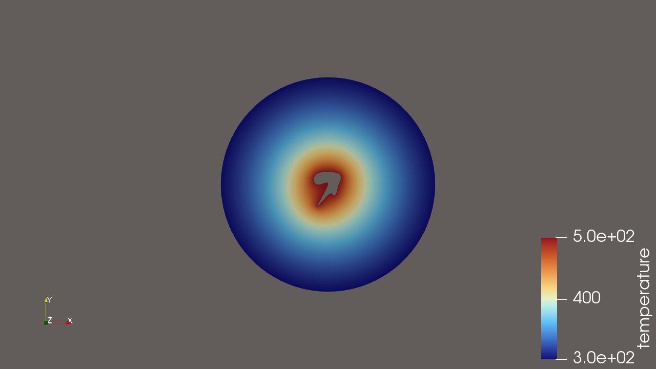
Once paraview launches, click ‘Apply’ inside the Properties tab on the left-hand side, then select ‘temperature’ under the Coloring section. The resulting Layout of the object should look something like this:
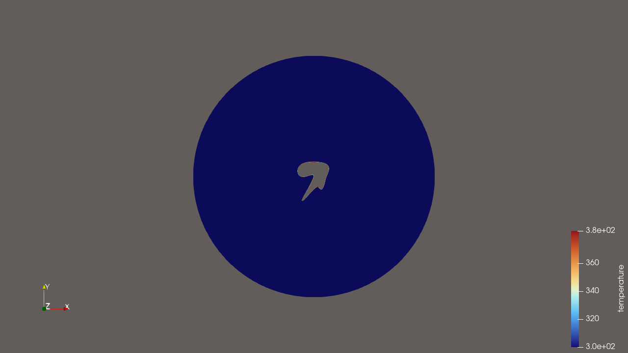
Now let’s see the output from the last time step, i.e. t=10s:
paraview test_vtk.10/Volume.vtu
Again, once paraview launches, click ‘Apply’ inside the Properties tab, then select ‘temperature’ under the Coloring section. You should see something like this: