FlowPsi
FlowPsi is an open-source Computational Fluid Dynamics (CFD) solver developed on top of the Loci framework by Dr. Ed Luke’s research group at Mississippi State University. For more information on FlowPsi, check out the following resources:
Official FlowPsi GitHub repository: LINK
In this demo, we will explore FlowPsi on Muscadine on a simple test case.
Loading FlowPsi on Muscadine
FlowPsi is built on top of Loci. Loading loci automatically loads FlowPsi and all associated dependencies:
module load loci/v4.2.a0
Verify the installation and version string:
flowpsi -v
Setting Up the Demo
In this demo, we will load the ‘cylinder’ example module that comes with FlowPsi, inspect the files, and then view the output after running.
Set up a demo folder in your local /scratch directory:
mkdir -p /scratch/hpc2/$USER/flowpsi_demo
cd /scratch/hpc2/$USER/flowpsi_demo
Copy the cylinder tutorial files from the FlowPsi installation:
cp $FLOWPSI_BASE/examples/cylinder/* .
Confirm the example files are present:
╰─$ ls
cylinder.vars  cylinder.vog
Inspecting files
Before running a CFD simulation, let’s check the quality of the grid for this example:
vogcheck cylinder
vogcheck provides a detailed assessment of quality measures. It also provides an overall assessment at the end, with excellent meaning ideal grid quality.
Next, let’s inspect the cylinder.vars file:
╰─$ cat cylinder.vars
{
boundary_conditions:<
 BC_1=symmetry, BC_2=symmetry,     // opposing slice faces
 BC_3=reflecting, BC_4=reflecting, // Two reflection walls
 BC_5=reflecting,                 // cylinder surface
 BC_6=farfield(T = 300K, p = 1atm, u=1m/s )
>
// Set reference pressure for gauge pressure output
// Note, this is needed for very low speed flows like this to get an
// accurte result
p0: 1atm

initialConditions  : < T = 300K, p = 1atm, u=1m/s>

flowRegime: inviscid
timeStepMode: steady

print_freq: 50
plot_freq:50
plot_modulo:50

restart_freq:50

restart_modulo:0
stop_iter: 100

// Take large time-steps, rely on urelax to keep things from getting out
// of hand
// Keep changes in P and T within reason, helps accellerate robustness
// of convergence by allowing larger timesteps.
urelax:  0.2
// If none of the above limits come into effect, take timesteps at
// 1 second intervals
dtmax:  1e1

limiter: none

fluidLinearSolver:lsgs

// low speed flow so setup pseudo timestepping and preconditioning controls
pseudo_cflmax: 10
Minf: 0.002

}
Our cylinder demo will run for 100 iterations as indicated by stop_iter, and solution output files are created every 50 iterations as indicated by plot_freq.
Running FlowPsi
Let’s do a quick flowpsi run for our example:
flowpsi cylinder
As FlowPsi executes, you can see the output residuals printed at every step.
Once this step is completed, output and restart directories are created.
Extracting Data for Visualization
Loci provides the extract utility to export raw datapoints into formats compatible with post-processing tools like ParaView.
Syntax
extract <tool> <caseName> <timeStep> [variable]
For more information on extract, simply type the following into your terminal:
extract
Viewing Results
For this demo, we will extract time steps into the VTK format. Let’s extract the data for t=0.
extract -vtk cylinder 0
Viewing Results in ParaView
Now that we extracted some data, let’s visualize them using Paraview.
Ensure Paraview is loaded first:
ml load paraview
Let’s see the output from the first time step, i.e. t=0s:
paraview cylinder_vtk.0/Volume.vtu
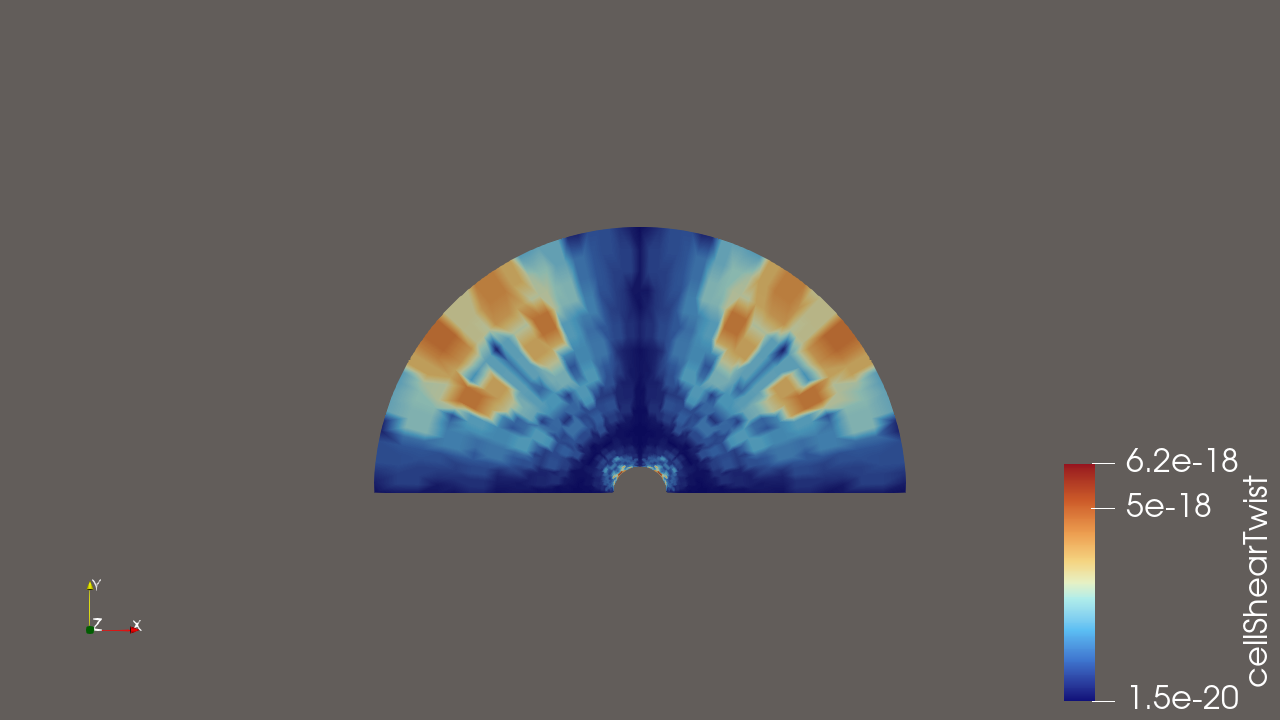
Once paraview launches, click ‘Apply’ inside the Properties tab on the left-hand side, then select any parameter under the Coloring section (in the image below, cellShearTwist was selected). The resulting Layout of the object should look something like this: